Backtrader: the fund

Already for a while, backtrader has been in use, so to say, professionally, besides the the known usage of backtrader some banks and trading houses, for the Backtrader Fund.

The history

A group of like-minded and long known to each other individuals decided to go down the road of opening a (Hedge) Fund and use backtrader as the foundation stone for the trading ideas. There was one thing which couldn’t be forgone: it had to be 100% regulated (but not in the Cayman Islands or a similar place)

Location, heritage and networking put the emphasis first in the European Union and then in Spain, where (as in some other places) the legislation allows for Umbrella Funds to host Sub-Funds, which enables creating a fully regulated fund with less money and number of participants.

And … the fund was approved by the CNMV (Comisión Nacional del Mercado de Valores), the regulating body in Spain with ISIN: ES0131444038. The links:

For those capable of reading Spanish, the usage of backtrader is documented in the official Fund leaflet.

And for those who may, at some point time, decide to go down the road, the most important things:

Bureaucracy is slow and there will be many questions along the road
Keep track of everything (operations executed, cash/net-asset-value levels, positions, leverage)
Reporting to the regulating body is a must (hence the need to collect and keep the aforementioned information well organized)
Keeping within the defined risk/volatility levels is not just a guideline
Managing OPM (Other People’s Money) is a real psychological burden. There will be losses and there will be questions. No matter how well intended and naive the questions may be: they have an impact.

backtrader is the foundation for the trading ideas and it has found a new field of application: reporting. Custom Analyzers and Indicators to keep control of the risk/volatility have eased the administrative burden.

Probably because we are old (and old fashioned) we still prefer manual execution (automated execution will sometime in the future take over)

The functionality described below was developed to aid in managing the fund and backtesting scenarios in which money goes in and out and performance is no longer a matter of tracking the net asset value.

Fund Tracking

With version 1.9.52.121, the broker in backtrader keeps track of the accounting not only in cash/value terms, but also as it would be done in a Fund, i.e.:

The value of the fund (of the fund shares actually)
The amount of shares

With this, one can actually simulate cash deposits and cash withdrawals, whilst still keeping track of the actual performance, which with a regular accounting would be distorted by the cash in/out-flows.

In addition to the changes in the broker, Analyzers and Observers have been adapted (those doing something with the net asset value) to support a fund parameter, to decide what should actually be tracked. For example TimeReturn:

...
cerebro.addanalyzer(bt.analyzers.TimeReturn)  # auto-detect broker mode
cerebro.addanalyzer(bt.analyzers.TimeReturn, fund=True)  # track fund value
cerebro.addanalyzer(bt.analyzers.TimeReturn, fund=False)  # track net asset value
...

What is this fund tracking?

Imagine the use case (later in the sample) of someone who starts with 1000 monetary units and on the 15^th of each month adds 100 monetary units. After 12 months, the total in the account is 2200. Returns calculated on a position taking initially

Calculating the returns in a usual way this would mean that without having executed a single operation, the performance in terms on annual returns is: 120%. Of course, this isn’t right.

To alleviate this problem and regardless of the initial value of the account, the value of the fund shares (fundvalue) is set to 100.0. And with that and the starting net asset value (the 1000 monetary units), one calculates the number of fund shares as

fundshares = net-asset-value / fundvalue

Which in this case is 1000 / 100.0 = 10 shares

With each cash addition, we increase the number of shares with:

new_fund_shares = cash_addition / fundvalue

Because we are adding 100.0 monetary units and no operation has been executed:

- ``100.0 / 100.0 = 1 share``

Notice that the fundvalue remains unchanged. Quickly forwarding to the end of the year we have the following:

Starting net-asset-value: 1000
Final net-asset-value: 2200
Starting fundvalue = 100
Final fundvalue = 100
Starting number of shares: 10
Final number of shares: 22

Now if we calculate the returns using the starting and ending fundvalues and because they are the same we have a: 0% which matches the reality. because cash additions have not changed

Using fund tracking in backtrader

Adding cash

First, the broker has gained a method to canonically add cash to the system:

add_cash(cash)

Using it inside the strategy for example:

def next(self):

    if whatever:
        self.broker.add_cash(1000.0)

This method MUST be used to track the entry and exit of cash into the system and properly track the fund value.

Automatic

Activate it in the broker:

...
cerebro.broker.set_fundmode(True)
...

changing at the same time the default fund start value:

...
cerebro.broker.set_fundmode(True, 10.0)  # the default is 100
...

or in independent calls:

...
cerebro.broker.set_fundmode(True)
cerebro.broker.set_fundstartval(10.0)  # the default is 100
...

After activation of the default mode and coming back to the TimeReturn analyzer examples from above:

...
# 1
cerebro.addanalyzer(bt.analyzers.TimeReturn)  # auto-detect broker mode
# 2
cerebro.addanalyzer(bt.analyzers.TimeReturn, fund=True)  # track fund value
# 3
cerebro.addanalyzer(bt.analyzers.TimeReturn, fund=False)  # track net asset value
...

1 and 2 are equivalent. But one should go for 1. If one wishes to compare, one can always force the TimeReturn analyzer to not use the fundvalue and rather track the net-asset-value

An example is worth a thousand words. In the sample, we’ll be using doing as described above but with some extra cash (the asset has a per-share value over 3000). The initial cash level will be 10000, the default in backtrader and on the 15^th of each month, 1000 extra monetary units will be added (using a recurring Timer). It will be 24 months (which is the size of the standard data sample used in backtrader)

Without any operations

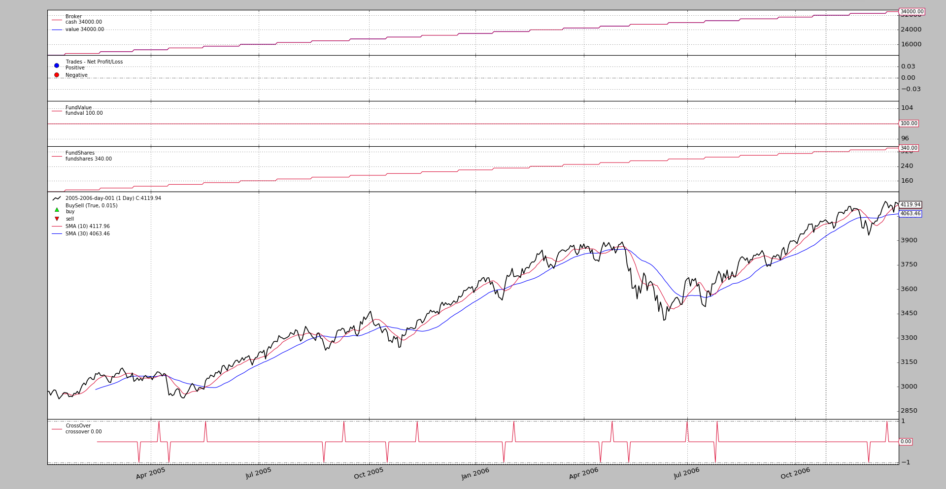
$ ./fund-tracker.py --broker fundmode=True --strat cash2add=1000 --cerebro writer=True --plot

The graphical view

And the text output (capped for readability):

- timereturn:
  ~~~~~~~~~~~~~~~~~~~~~~~~~~~~~~~~~~~~~~~~~~~~~~~~~~~~~~~~~~~~~~~~~~~~~
    ...
    - fund: None
  ~~~~~~~~~~~~~~~~~~~~~~~~~~~~~~~~~~~~~~~~~~~~~~~~~~~~~~~~~~~~~~~~~~~~~
  - Analysis:
    - 2005-12-31: 0.0
    - 2006-12-31: 0.0
.......................................................................
- timereturn1:
  ~~~~~~~~~~~~~~~~~~~~~~~~~~~~~~~~~~~~~~~~~~~~~~~~~~~~~~~~~~~~~~~~~~~~~
  - Params:
    ...
    - fund: True
  ~~~~~~~~~~~~~~~~~~~~~~~~~~~~~~~~~~~~~~~~~~~~~~~~~~~~~~~~~~~~~~~~~~~~~
  - Analysis:
    - 2005-12-31: 0.0
    - 2006-12-31: 0.0
.......................................................................
- timereturn2:
  ~~~~~~~~~~~~~~~~~~~~~~~~~~~~~~~~~~~~~~~~~~~~~~~~~~~~~~~~~~~~~~~~~~~~~
    ...
    - fund: False
  ~~~~~~~~~~~~~~~~~~~~~~~~~~~~~~~~~~~~~~~~~~~~~~~~~~~~~~~~~~~~~~~~~~~~~
  - Analysis:
    - 2005-12-31: 1.2
    - 2006-12-31: 0.545454545455

There are 3 TimeReturn analyzers getting added.

The 1^st has fund=None (default) which means to track the actual fundmode set in the broker (in this case True)

It says that the yearly returns were 0.0 and 0.0. Since we made no operations: Ok
The 2^nd has fund=True which means to use the fundvalue always

It says that the yearly returns were 0.0 and 0.0. Since we made no operations: Ok
The 3^rd has fund=False which means to use the net-asset-value always

It says that the yearly returns were 1.2 (120%) and 0.54 (54%). Since we made no operations: This is clearly wrong

The plot contains also the 2 new Observers (FundValue and FundShares) which allow to see how even if the net-asset-value grows with the addition of cash every month, the fundvalue remains constant as 100.0. At the same times the shares grow with each cash addition.

Let’s trade

The same as above but with some trading using a standard moving average crossover

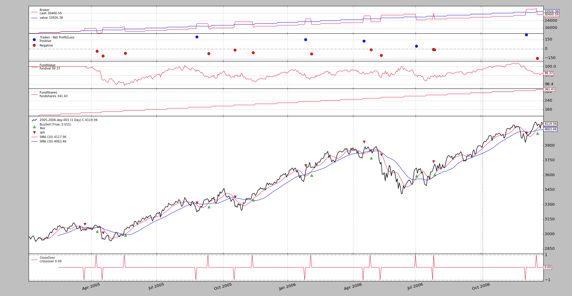
$ ./fund-tracker.py --broker fundmode=True --strat cash2add=1000,trade=True --cerebro writer=True --plot

The graphical view

And the text output (capped for readability):

- timereturn:
    ...
    - fund: None
  ~~~~~~~~~~~~~~~~~~~~~~~~~~~~~~~~~~~~~~~~~~~~~~~~~~~~~~~~~~~~~~~~~~~~~
  - Analysis:
    - 2005-12-31: -0.00642229824537
    - 2006-12-31: 7.78998679263e-05
.......................................................................
- timereturn1:
    ...
    - fund: True
  ~~~~~~~~~~~~~~~~~~~~~~~~~~~~~~~~~~~~~~~~~~~~~~~~~~~~~~~~~~~~~~~~~~~~~
  - Analysis:
    - 2005-12-31: -0.00642229824537
    - 2006-12-31: 7.78998679263e-05
.......................................................................
- timereturn2:
  ~~~~~~~~~~~~~~~~~~~~~~~~~~~~~~~~~~~~~~~~~~~~~~~~~~~~~~~~~~~~~~~~~~~~~
    ...
    - fund: False
  ~~~~~~~~~~~~~~~~~~~~~~~~~~~~~~~~~~~~~~~~~~~~~~~~~~~~~~~~~~~~~~~~~~~~~
  - Analysis:
    - 2005-12-31: 1.19378185337
    - 2006-12-31: 0.546479045423

The same three TimeReturn analyzers from before. The ones with fund=None and fund=True give reasonable results whereas the one using fund=False is clearly off the chart again with 119% and 54%, which is clearly not the return offered by the moving average crossover.

Manual

In this case (which is the default in the broker and even if the broker is tracking the value of the fund, only those analyzers with fund=True will use the value.

A quick run with only the textual ouput:

$ ./fund-tracker.py --strat cash2add=1000,trade=True --cerebro writer=True

Output:

- timereturn:
  ~~~~~~~~~~~~~~~~~~~~~~~~~~~~~~~~~~~~~~~~~~~~~~~~~~~~~~~~~~~~~~~~~~~~~
    ...
    - fund: None
  ~~~~~~~~~~~~~~~~~~~~~~~~~~~~~~~~~~~~~~~~~~~~~~~~~~~~~~~~~~~~~~~~~~~~~
  - Analysis:
    - 2005-12-31: 1.19378185337
    - 2006-12-31: 0.546479045423
.......................................................................
- timereturn1:
  ~~~~~~~~~~~~~~~~~~~~~~~~~~~~~~~~~~~~~~~~~~~~~~~~~~~~~~~~~~~~~~~~~~~~~
    ...
    - fund: True
  ~~~~~~~~~~~~~~~~~~~~~~~~~~~~~~~~~~~~~~~~~~~~~~~~~~~~~~~~~~~~~~~~~~~~~
  - Analysis:
    - 2005-12-31: -0.00642229824537
    - 2006-12-31: 7.78998679263e-05
.......................................................................
- timereturn2:
  ~~~~~~~~~~~~~~~~~~~~~~~~~~~~~~~~~~~~~~~~~~~~~~~~~~~~~~~~~~~~~~~~~~~~~
    ...
    - fund: False
  ~~~~~~~~~~~~~~~~~~~~~~~~~~~~~~~~~~~~~~~~~~~~~~~~~~~~~~~~~~~~~~~~~~~~~
  - Analysis:
    - 2005-12-31: 1.19378185337
    - 2006-12-31: 0.546479045423

Now only the TimeReturn with fund=True delivers sensible results.

Conclusion

The new fundmode implemented in the broker and which can be used (automatically/manually) in the analyzers, allows to use backtrader to model the inner workings of a real fund or use cases like constant investment of money at given intervals.

Sample Usage

$ ./fund-tracker.py --help
usage: fund-tracker.py [-h] [--data0 DATA0] [--fromdate FROMDATE]
                       [--todate TODATE] [--cerebro kwargs] [--broker kwargs]
                       [--sizer kwargs] [--strat kwargs] [--plot [kwargs]]

Fund Tracking Sample

optional arguments:
  -h, --help           show this help message and exit
  --data0 DATA0        Data to read in (default:
                       ../../datas/2005-2006-day-001.txt)
  --fromdate FROMDATE  Date[time] in YYYY-MM-DD[THH:MM:SS] format (default: )
  --todate TODATE      Date[time] in YYYY-MM-DD[THH:MM:SS] format (default: )
  --cerebro kwargs     kwargs in key=value format (default: )
  --broker kwargs      kwargs in key=value format (default: )
  --sizer kwargs       kwargs in key=value format (default: )
  --strat kwargs       kwargs in key=value format (default: )
  --plot [kwargs]      kwargs in key=value format (default: )

Sample Code

from __future__ import (absolute_import, division, print_function,
                        unicode_literals)

import argparse
import datetime

import backtrader as bt


class St(bt.SignalStrategy):
    params = dict(
        cash2add=None,
        cashonday=15,
        pfast=10,
        pslow=30,
        trade=False,
    )

    def __init__(self):
        self.add_timer(when=bt.Timer.SESSION_END, monthdays=[self.p.cashonday])

        sma1 = bt.ind.SMA(period=self.p.pfast)
        sma2 = bt.ind.SMA(period=self.p.pslow)
        signal = bt.ind.CrossOver(sma1, sma2)
        if self.p.trade:
            self.signal_add(bt.SIGNAL_LONGSHORT, signal)

    def notify_timer(self, timer, when, *args, **kwargs):
        # no need to check the timer, there is only one
        if self.p.cash2add is not None:
            self.broker.add_cash(self.p.cash2add)

    def next(self):
        pass


def runstrat(args=None):
    args = parse_args(args)

    cerebro = bt.Cerebro()

    # Data feed kwargs
    kwargs = dict()

    # Parse from/to-date
    dtfmt, tmfmt = '%Y-%m-%d', 'T%H:%M:%S'
    for a, d in ((getattr(args, x), x) for x in ['fromdate', 'todate']):
        if a:
            strpfmt = dtfmt + tmfmt * ('T' in a)
            kwargs[d] = datetime.datetime.strptime(a, strpfmt)

    data0 = bt.feeds.BacktraderCSVData(dataname=args.data0, **kwargs)
    cerebro.adddata(data0)

    # Broker
    cerebro.broker = bt.brokers.BackBroker(**eval('dict(' + args.broker + ')'))

    # Sizer
    cerebro.addsizer(bt.sizers.PercentSizer,
                     **eval('dict(' + args.sizer + ')'))

    # Strategy
    cerebro.addstrategy(St, **eval('dict(' + args.strat + ')'))

    cerebro.addobserver(bt.observers.FundValue)
    cerebro.addobserver(bt.observers.FundShares)

    ankwargs = dict(timeframe=bt.TimeFrame.Years)
    cerebro.addanalyzer(bt.analyzers.TimeReturn, **ankwargs)
    cerebro.addanalyzer(bt.analyzers.TimeReturn, fund=True, **ankwargs)
    cerebro.addanalyzer(bt.analyzers.TimeReturn, fund=False, **ankwargs)

    # Execute
    cerebro.run(**eval('dict(' + args.cerebro + ')'))

    if args.plot:  # Plot if requested to
        cerebro.plot(**eval('dict(' + args.plot + ')'))


def parse_args(pargs=None):
    parser = argparse.ArgumentParser(
        formatter_class=argparse.ArgumentDefaultsHelpFormatter,
        description=(
            'Fund Tracking Sample'
        )
    )

    parser.add_argument('--data0', default='../../datas/2005-2006-day-001.txt',
                        required=False, help='Data to read in')

    # Defaults for dates
    parser.add_argument('--fromdate', required=False, default='',
                        help='Date[time] in YYYY-MM-DD[THH:MM:SS] format')

    parser.add_argument('--todate', required=False, default='',
                        help='Date[time] in YYYY-MM-DD[THH:MM:SS] format')

    parser.add_argument('--cerebro', required=False, default='',
                        metavar='kwargs', help='kwargs in key=value format')

    parser.add_argument('--broker', required=False, default='',
                        metavar='kwargs', help='kwargs in key=value format')

    parser.add_argument('--sizer', required=False, default='',
                        metavar='kwargs', help='kwargs in key=value format')

    parser.add_argument('--strat', required=False, default='',
                        metavar='kwargs', help='kwargs in key=value format')

    parser.add_argument('--plot', required=False, default='',
                        nargs='?', const='{}',
                        metavar='kwargs', help='kwargs in key=value format')

    return parser.parse_args(pargs)


if __name__ == '__main__':
    runstrat()