Canonical vs Non-Canonical Indicators

The question has shown up several times more or less like this:

How is this or that best/canonically implemented with backtrader?

Being one of the goals of backtrader to be flexible to support as many situations and use cases as possible, the answer is easy: "In at least a couple of ways". Summarized for indicators, for which the question most often happens:

100% declarative in the __init__ method
100% step-by-step in the next method
Mixing both of the above for complex scenarios in which the declarative part cannot cover all needed calculations

A quick view of the built-in indicators in backtrader reveals that all of them are implemented in a declarative manner. The reasons

Easier to do
Easier to read
More elegant
Vectorized and even-based implementations are automatically managed

What ?!?! Auto-implemented Vectorization??

Yes. If an indicator is implemented entirely inside the __init_ method, the magic of metaclasses and operator overloading in Python will deliver the following

A vectorized implementation (default setting when running a backtest)
An event-based implementation (for example for live trading)

On the other hand and if any part of an indicator which is implemented in the next method:

This is the code directly used for an event-based run.
Vectorization will be simulated by calling the next method in the background for each data point

Note

This means that even if a particular indicator does not have a vectorized implementation, all others which have it, will still run vectorized

Money Flow Index: an Example

Community User @Rodrigo Brito posted a version of the "Money Flow Index" indicator which used the next method for the implementation.

The code

Non Canonical MFI Implementation

class MFI(bt.Indicator):
    lines = ('mfi', 'money_flow_raw', 'typical', 'money_flow_pos', 'money_flow_neg')

    plotlines = dict(
        money_flow_raw=dict(_plotskip=True),
        money_flow_pos=dict(_plotskip=True),
        money_flow_neg=dict(_plotskip=True),
        typical=dict(_plotskip=True),
    )

    params = (
        ('period', 14),
    )

    def next(self):
        typical_price = (self.data.close[0] + self.data.low[0] + self.data.high[0]) / 3
        money_flow_raw = typical_price * self.data.volume[0]

        self.lines.typical[0] = typical_price
        self.lines.money_flow_raw[0] = money_flow_raw

        self.lines.money_flow_pos[0] = money_flow_raw if self.lines.typical[0] >= self.lines.typical[-1] else 0
        self.lines.money_flow_neg[0] = money_flow_raw if self.lines.typical[0] <= self.lines.typical[-1] else 0

        pos_period = math.fsum(self.lines.money_flow_pos.get(size=self.p.period))
        neg_period = math.fsum(self.lines.money_flow_neg.get(size=self.p.period))

        if neg_period == 0:
            self.lines.mfi[0] = 100
            return

        self.lines.mfi[0] =  100 - 100 / (1 +  pos_period / neg_period)

Note

Kept as originally posted including the long lines for which one has to scroll horizontally

@Rodrigo Brito already notices that the usage of temporary lines is (all lines except mfi) is something which probably admits optimization. Indeed, but in the humble opinion of the author*, actually everything does admit a bit of optimization.

To have common working grounds, one can use the "Money Flow Index" definition by StockCharts and see that the implementation above is good. Here is the link:

https://school.stockcharts.com/doku.php?id=technical_indicators:money_flow_index_mfi

With that in the hand, a quick Canonical implementation of the MFI indicator

Canonical MFI Implementation

class MFI_Canonical(bt.Indicator):
    lines = ('mfi',)
    params = dict(period=14)

    def __init__(self):
        tprice = (self.data.close + self.data.low + self.data.high) / 3.0
        mfraw = tprice * self.data.volume

        flowpos = bt.ind.SumN(mfraw * (tprice > tprice(-1)), period=self.p.period)
        flowneg = bt.ind.SumN(mfraw * (tprice < tprice(-1)), period=self.p.period)

        mfiratio = bt.ind.DivByZero(flowpos, flowneg, zero=100.0)
        self.l.mfi = 100.0 - 100.0 / (1.0 + mfiratio)

One should be able to immediately notice

A single line mfi is defined. No temporaries are there.
Things seem cleaner with no need for [0] array indexing
No single if here or there
More compact whilst more readable

Should one plot a graph of both run against the same data set, it would look like this

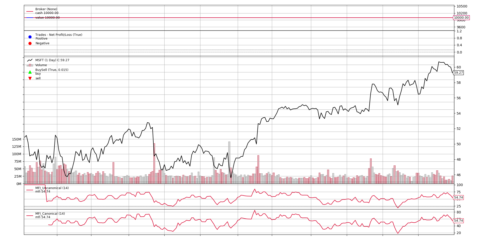
The chart shows that both the Canonical and Non-Canonical versions show the same values and development, except at the beginning.

The Non-Canonical version is delivering values from the very start
It is delivering non-meaningful values (100.0 until it deliver 1 extra value which is also not good) because it cannot properly deliver

In contrast:

The Canonical version automatically starts delivering values after the minimum warm-up period has been reached.
No human intervention has been needed (it must for sure be "Articifial Intelligence" or "Machine Learning", ... pun intended)

See a close-up picture of the affected area

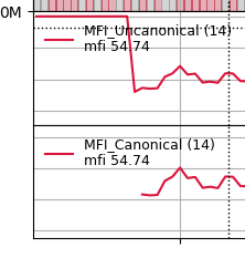
Note

One could of course try to alleviate this situation in the Non-Canonical version by doing this:

Subclassing from bt.ind.PeriodN which already has a period param and knows what to do with it (and calling super during __init__)

Notice also that the Canonical version does also account, like the step-by-step next code for a possible division-by-zero situation in the formula.

Non Canonical Division By Zero Handling

        if neg_period == 0:
            self.lines.mfi[0] = 100
            return

        self.lines.mfi[0] =  100 - 100 / (1 +  pos_period / neg_period)

whereas this is the other way to do it

Canonical Division By Zero Handling

        mfiratio = bt.ind.DivByZero(flowpos, flowneg, zero=100.0)
        self.l.mfi = 100.0 - 100.0 / (1.0 + mfiratio)

Instead of having many lines, a return statement and different assignments to the output line, there is s single declaration of the mfiratio calculation and a single assignment (following the StockCharts formula) to the output line mfi.

Conclusion

Hopefully, this sheds some light as to what the differences can be when implementing something in the Canonical (i.e.: declarative in __init_) or Non-Canonical way (step by step with array indexing in next)